Table of Contents

1. Introduction
2. Motivation
3. Process Modeling
   1. Linear Gaussian Dynamic Bayesian Network Based Hybrid Model
      1. Process Trajectory/Episode Distribution
      2. Model Formulation
      3. Inference
   2. Nonlinear Dynamic Bayesian Network Based Hybrid Model
      1. Parametric Variation Modeling
      2. Latent State Modeling
      3. Inference (A Bayesian Approach)
4. Conclusion
5. Next?
6. Reference

Introduction

This is a tutorial about a series of advanced hybrid process models for people with some background in mathematical and statistical modeling and interested in the process modeling. The class of process models I will present in this tutorial is mainly based on Bayesian network and Bayesian inference.

Motivation

For many biochemical/physical/economic processes, the laws of physics and biochemistry often allow us to construct mechanistic models in forms of ordinary/partial/algebraic differential equations. While these models can well describe the the mean changes in a reaction/movement/economy profile over time, these models often ignore the impact from various sources of process inherent stochasticity. For example, in a cell culture process, although batch-to-batch variation and bioprocess noise are often dominant sources of process variation [1], biochemical kinetics literature rarely incorporates them into the ordinary/partial differential equation (ODE/PDE) based mechanistic models. In a study on the microbial cell-to-cell phenotypic diversity, [2] identified the intracellular production fluctuations as one of the major sources of the bioprocessing noise. Raw material variability is another critical source of uncertainty impacting cell cultures [3]. In fact, process noises are widely seen in most complex systems such as economy, cell metabolism, production process of mRNA vaccines. Therefore, it is of great importance to understand and incorporate major sources of stochastic uncertainty into a process model.

Process Modeling

Process-based modeling is a modeling framework for complex systems. In contrast to agent-based models and other mainstream languages in complex systems, in a process-based model the structural features of a system are encoded in the interactions between the entities, rather than in the entities themselves.

Ordinary Differential Equations Based Mechanistic Model

A control system is a dynamical system on which one can act by using suitable controls. In this article, the dynamical model is modeled by ordinary differential equations of the following type

$$ \dot{\pmb{s}}=\pmb f(\pmb s,\pmb a)\tag{1}\label{eq: 1} $$ where $\pmb{f}(\cdot)$ encodes the causal interdependencies between actions and state. One typically assumes that the functional form of $\pmb{f}$ is known, though it may also depend on additional parameters calibrated from data. The variable $\pmb s$ is the state and belongs to some space $\mathcal{S}$. The variable $\pmb{a}$ is the control and belongs to some space $\mathcal{A}$. In this article, the space $\mathcal{S}$ is of infinite dimension.

Remark:

1. In control literature, people use the state and control variables $(x,u)$ instead of state and action $(\pmb{s},\pmb{a})$.
2. This is a first order differential equation;
3. $\pmb f(\cdot)=\left(f_1,\ldots, f_n\right)(\cdot)=\left(f_1(\cdot),\ldots, f_n(\cdot)\right)$ is a vector of functions.
4. Some characteristics of the dynamical system can be used to analyze the Eq.(1), such as
   • Stability: means that the trajectories do not change too much under small perturbations.
   • Asymptotically stability
   • controllability:

Example: the kinetic/dynamic equations is linear, e.g. $\dot{s}=\mu s(t)$, where $\mu$ is a constant, and in this case, $f(x)=ax$. The stability of linear systems is straightforward, i.e. stable if $\mu<0$, and unstable otherwise.

Linear Gaussian Dynamic Bayesian Network Based Hybrid Model [4]

We model the process dynamics as a finite-horizon Markov decision process (MDP) specified by $(\mathcal{S}, \mathcal{A}, H, r, p)$, where $\mathcal{S}$, $\mathcal{A}$, $H$, $r$ and $p$ represent state space, action space, planning horizon, reward function, and state transition probability model. The process state transition is modeled as, $$ \begin{equation} \pmb{s}_{t+1} \sim p(\pmb{s}_{t+1}|\pmb{s}_t,\pmb{a}_t;\pmb\theta_t) \end{equation} $$

where $\pmb{s}_t\in \mathcal{S}\subset \mathbb{R}^n$ denotes the process state (e.g., glucose and lactate concentrations and cell density), $\pmb{a}_t \in \mathcal{A}\subset\mathbb{R}^m$ is the action (also known as control inputs) at time step $t\in\mathcal{H}$. Here $\mathcal{H}\equiv{1,2,\ldots,H}$ denotes the discrete time index (a.k.a. decision epochs).

Process Trajectory/Episode Distribution

Then, the distribution of the entire trajectory $\pmb\tau=(\pmb{s}_1,\pmb{a}_1,\pmb{s}_2,\pmb{a}_2,\ldots,\pmb{s}_{H})$ of the process can be written as a product

$$ p(\pmb{\tau}) = p(\pmb{s}_1)\prod_{t=1}^{H-1} p(\pmb{s}_{t+1}|\pmb{s}_t,\pmb{a}_t) p(\pmb{a}_t)\tag{2}\label{eq:trajectory-distribution} $$ of conditional distributions. Given a set of real-world process observations denoted by $\mathcal{D} =\left\{\pmb\tau^{(n)}\right\}^N_{n=1}$, we quantify the model parameter estimation uncertainty using the posterior distribution $p(\pmb{\theta}|\mathcal{D})$.

Model Formulation

Suppose that $\pmb s_t$ evolves according to the ordinary differential equation \eqref{eq: 1} and the dynamics is monitored on a small time scale using sensors, let us replace Eq. \eqref{eq: 1} by the first-order Taylor approximation

$$ \begin{equation} \frac{\Delta \pmb{s}_{t+1}}{\Delta t} =\pmb{f}(\pmb\mu_t^s,\pmb\mu_t^a)+J^s_f(\pmb\mu_t^s)(\pmb{s}_t-\pmb\mu_t^s)+J^a_f(\pmb\mu_t^a)(\pmb{a}_t-\pmb\mu_t^a), \tag{3}\label{eq:taylor1} \end{equation} $$ where $\Delta \pmb{s}_{t+1}=\pmb{s}_{t+1}-\pmb{s}_{t}$, and $J^s_f,J^a_f$ denote the Jacobian matrices of $\pmb{f}$ with respect to $\pmb{s}_t$ and $\pmb{a}_t$, respectively. The interval $\Delta t$ can change with time, but we keep it constant for simplicity. The approximation is taken at a point $\left(\pmb\mu_t^s,\pmb\mu_t^a\right)$. We can then rewrite Eq. \eqref{eq:taylor1} as

$$ \begin{equation} \scriptsize \pmb{s}_{t+1} = \pmb{\mu}_{t}^s + \Delta t\cdot \pmb{f}(\pmb\mu_t^s,\pmb\mu_t^a)+(\Delta t \cdot J_f(\pmb\mu_t^s)+1)(\pmb{s}_t-\pmb\mu_t^s)+\Delta t \cdot J_f(\pmb\mu_t^a)(\pmb{a}_t-\pmb\mu_t^a)+R_{t+1}\tag{4}\label{eq:taylor} \end{equation} $$

where $R_{t+1}$ is a remainder term modeling the effect from other uncontrolled factors. In this way, the original process dynamics have been linearized, with $R_{t+1}$ serving as a residual. One can easily represent Eq. \eqref{eq:taylor} using a network model. An edge exists from $s^k_t$ (respectively, $a^k_t$) to $s^l_{t+1}$ if the $\left(k,l\right)$-th entry of $J^s_f$ (respectively, $J^a_f$) is not identically zero.

As will be seen shortly, the linearized dynamics can be rewritten in a linear Gaussian dynamic Bayesian network. Specifically, let

$$ \begin{align*}\pmb\mu_{t+1}^s &=\pmb{\mu}_{t}^s + \Delta t\cdot \pmb{f}(\pmb\mu_t^s,\pmb\mu_t^a),\\ \pmb\beta_{t}^s &= \Delta t \cdot J_f(\pmb\mu_t^s)+1,\\ \pmb\beta_{t}^a &=\Delta t \cdot J_f(\pmb\mu_t^a),\end{align*} $$

and treat $R_{t+1}$ as the residual $\pmb{e}_{t+1}=V_{t+1}^{1/2}\pmb{z}$, with $\pmb{z}$ is an $n$-dimensional standard normal random vector, and $V_{t+1}\triangleq\text{diag}(v_{t+1}^{k})$ is a diagonal matrix of residual standard deviation. we can turn Eq. \eqref{eq:taylor} into a Linear Gaussian (Dynamic) Bayesian Network [5]:

$$ \begin{equation} \pmb{s}_{t+1} = \pmb{\mu}_{t+1}^s + \left(\pmb{\beta}_{t}^s\right)^\top(\pmb{s}_t-\pmb\mu_t^s) + \left(\pmb\beta_{t}^a\right)^\top(\pmb{a}_t-\pmb\mu_t^a) +V_{t+1}^{1/2}\pmb{z}_{t+1}\tag{5}\label{eq: 5} \end{equation} $$ where

• $s_t\in\mathcal{S}\subset \mathbb{R}^n, \pmb{a}_t\in\mathcal{A}\subset \mathbb{R}^{m}$
• $\pmb\mu_{t}^s=(\mu_t^{1},\ldots, \mu_t^n)$ and $\pmb\mu_{t}^a=(\lambda_t^{1},\ldots, \lambda_t^m)$ ,
• $\pmb\beta_{t}^s$ is the $n\times n$ matrix whose $\left(j,k\right)$-th element is the linear coefficient $\beta^{jk}_t$ corresponding to the effect of state $s^j_t$ on the next state $s^k_{t+1}$
• $\pmb\beta_t^a$ is the $m\times n$ matrix of analogous coefficients representing the effects of each component of $\pmb{a}_t$ on each component of $\pmb{s}_{t+1}$.

State transition: From Eq.\eqref{eq: 5}, the state transition becomes $$ \begin{equation*}\small \pmb{s}_{t+1} \sim p(\pmb{s}_{t+1}|\pmb{s}_t,\pmb{a}_t;\pmb\theta_t)=\mathcal{N}\left( \pmb{\mu}_{t+1}^s + \left(\pmb{\beta}_{t}^s\right)^\top(\pmb{s}_t-\pmb\mu_t^s) + \left(\pmb\beta_{t}^a\right)^\top(\pmb{a}_t-\pmb\mu_t^a), V_{t+1}\right) \end{equation*} $$ with $\pmb\theta_t=(\pmb{\mu}_{t+1}^s,\pmb\mu_t^s,\pmb\mu_t^a,\pmb{\beta}_{t}^s, \pmb\beta_{t}^a, V_{t+1})$.

Initial State: $\pmb{s}_1\sim \mathcal{N}(\pmb\mu^s_1,V_1)$ or $s_{1}^k \sim \mathcal{N}(\mu^k_{1},(v^k_{1})^2)$ for $k=1,2,\ldots,m$.

Action: $\pmb{a}_t\sim\mathcal{N}\left(\pmb\mu^a_t,\text{diag}(\sigma_t^k)\right)$ or $a_{t}^k \sim \mathcal{N}(\lambda^k_{t},(\sigma^k_{t})^2)$ for $k=1,2,\ldots,m$

Parameters: Letting $\pmb\sigma_t=(\sigma_t^1,\ldots,\sigma_t^m)$ and $\pmb{v}_t=(v_t^1,\ldots,v_t^n)$, the list of parameters for full model is $$ \pmb{\theta} = (\pmb{\mu}^s,\pmb\mu^a,\pmb{\beta},\pmb\sigma,\pmb{v})= \{(\pmb{\mu}_{t}^s,\pmb\mu_t^a,\pmb{\beta}_{t}^s,\pmb\beta_{t}^a,\pmb\sigma_t,\pmb{v}_t)| 0\leq t\leq H\} $$ where $\pmb\beta = (\pmb\beta^a,\pmb\beta^s)$. Next, we will discuss how to estimate parameters $\pmb{\theta}$ from data.

Remark:

• $\pmb{v}_t$ is the diagonal (vector)of the diagonal covariance matrix $V_t$, i.e. $\pmb{v}_t=\text{diag}(V_{t})$.
• Action can be modeled by a policy distribution $\pmb{a}_t\sim \pi(\pmb{a}_t|\pmb{s}_t)$. This policy $\pi$ can be obtained from RL algorithms.

Inference

Bayesian Approach (See details in Appendix Section 10 of [4]):

• Full likelihood and conjugate prior

  Given the data $\mathcal{D}$, the posterior distribution of $\pmb{\theta}$ is proportional to $\pmb{\theta}$$p(\pmb\theta|\mathcal{D})\propto p\left(\pmb{\theta}\right)\prod_{n=1}^Np\left(\pmb{\tau}^{(n)}|\pmb{\theta}\right)$$.

  The Gibbs sampling technique can be used to sample from this distribution.

  For each node $X$ in the network, let $\text{Ch}\left(X\right)$ be the set of child nodes (direct successors) of $X$. The full likelihood $p\left(\mathcal{D}|\pmb{\theta}\right)$ becomes

  $$ \begin{equation*}\scriptsize p(\mathcal{D}|\pmb{\theta})=\prod^N_{i=1}p(\pmb{\tau}_i|\pmb{\theta})=\prod^N_{i=1}\prod_{t=1}^H\left[\prod_{k=1}^{m}\mathcal{N}\left(\lambda^k_{t},(\sigma^k_{t})^2\right)\prod_{k=1}^{n}\mathcal{N}\left(\mu^k_{t+1} + \sum_{X^j_t\in Pa(s^k_{t+1})}\beta^{jk}_{t}(X^j_t - \mu^j_t),(v^k_{t+1})^2\right)\right], \end{equation*} $$

  For the parameters $\pmb\mu^a, \pmb \mu^s,\pmb\sigma^2 \pmb v^2, \pmb \beta$, we have the conjugate prior $$ \begin{equation*}\small p(\pmb \mu^a, \pmb \mu^s,\pmb\sigma^2 \pmb v^2, \pmb \beta) = \prod_{t=1}^H\left(\prod_{k=1}^{m} p(\lambda^k_t)p\left((\sigma_k^{t})^2\right)\prod_{k=1}^{n} p(\mu^k_t)p\left((v^k_{t})^2\right) \prod_{i\neq j} p(\beta^{ij}_t)\right), \end{equation*} $$ where $$ \begin{equation} \small \begin{split} &p(\lambda^k_t) =\mathcal{N}\left({\lambda}^{k(0)}_t, \left({\delta}_{t,k}^{(\lambda)}\right)^2\right), \quad p(\mu^k_t) = \mathcal{N}\left({\mu}^{k(0)}_t, \left({\delta}_{t,k}^{(\mu)}\right)^2\right), \\ & p(\beta_{t}^{ij}) = \mathcal{N}\left({\beta}_{t}^{ij(0)}, \left({\delta}_{t,ij}^{(\beta)}\right)^2\right)\quad p\left((\sigma_t^k)^2\right) = \text{Inv-}\Gamma\left(\dfrac{\kappa_{t,k}^{(\sigma)}}{2}, \dfrac{\rho_{t,k}^{(\sigma)}}{2}\right), \\ &p((v_t^k)^2) = \text{Inv-}\Gamma\left(\dfrac{\kappa_{t,k}^{(v)}}{2}, \dfrac{\rho_{t,k}^{(v)}}{2}\right), \end{split} \end{equation} $$ where $\text{Inv-}\Gamma$ denotes the inverse-gamma distribution. We omit the tedious derivation for the posterior conditional distribution for each model parameters but you can find them in Appendix Section 10 of [4].

Frequentists’ Approach

Following [5] (p.318, Chapter 10), we can write the LG-DBN Eq.\eqref{eq: 5} as

$$ \begin{equation}\pmb\tau-\pmb\mu=B(\pmb\tau-\pmb\mu) - \Sigma^{1/2} \pmb u \tag{6}\label{eq: 6}\end{equation} $$ where $\pmb{\mu} = [\pmb{\mu}^s_1,\pmb{\mu}^a_1,\ldots,\pmb{\mu}^s_{H},\pmb{\mu}^a_{H},\pmb{\mu}^s_{H+1}]^\top$, $\pmb u$ is an $\left((H+1)n+Hm\right)$-dimensional standard normal random vector, $\Sigma^{\frac{1}{2}}=\text{diag}\left(\pmb{v}^s_1,\pmb\sigma_1,\ldots,\pmb{v}^s_H,\pmb\sigma_H,\pmb{v}^s_{H+1}\right)$ is the diagonal matrix of the conditional standard deviations of state and actions, and the coefficient matrix of observed trajectory is written as $$ B = \begin{bmatrix} 0 & 0 & 0 & 0 & 0 & 0 & \cdots & 0 & 0 & 0 & 0 \\0 & 0 & 0 & 0 & 0 & 0 & \cdots & 0 & 0 & 0 & 0\\\pmb{\beta}^s_1 & \pmb{\beta}^a_1 & 0 & 0 & 0 & 0 & \cdots & 0 & 0 & 0 & 0\\0 & 0 & 0 & 0 & 0 & 0 & \cdots & 0 & 0 & 0 & 0\\0 & 0& \pmb{\beta}^s_2 & \pmb{\beta}^a_2 & 0 & 0 &\cdots & 0 & 0 & 0 & 0\\0 & 0 & 0 & 0 & 0 & 0 & \cdots & 0 & 0 & 0 & 0\\\vdots & \vdots & \vdots & \vdots & \vdots & \vdots & \vdots & \vdots & \vdots & \vdots & \vdots\\ 0 & 0 & 0 & 0 & 0 & 0 & \cdots & \pmb{\beta}^s_H & \pmb{\beta}^a_H & 0 & 0\\\end{bmatrix} $$

Thus, by rearranging Eq.\eqref{eq: 6} and letting $\pmb{\tau}-\pmb\mu=(I-B)^{-1}\Sigma^{\frac{1}{2}} \pmb{u}$, we have $$ \pmb{\tau}\sim \mathcal{N}\left(\pmb\mu, (I-B)^{-1}\Sigma (I-B)^{-\top}\right) $$ with mean $\mathbb{E}[\pmb\tau]=\pmb{\mu}$ and covariance matrix $\text{Cov}\left(\pmb{\tau}-\pmb\mu\right)=(I-B)^{-1}\Sigma(I-B)^{-\top}$.

Estimating $\pmb\mu$:

Let $\tilde{\pmb\tau} \equiv (\tilde{\pmb{s}}_1,\tilde{\pmb{a}}_1,\ldots,\tilde{\pmb{s}}_H,\tilde{\pmb{a}}_H, \tilde{\pmb{s}}_{H+1}) =\pmb{\tau} - \pmb\mu$, where $\tilde{\pmb{s}}_t$ and $\tilde{\pmb{a}}_t$ denote centered observable state and decision. The unbiased estimator $\hat{\pmb\mu}=\frac{1}{N}\sum^N_{i=1}\pmb\tau^{(i)}$ can be easily obtained by using the fact $\mathbb{E}[\pmb\tau]=\pmb\mu$.

Estimating $\pmb\beta_t^s,\pmb\beta_t^a,\Sigma$:

The log-likelihood of the centered trajectory observations $\{\tilde{\pmb{\tau}}^{(i)}\}_{i=1}^N$ is, $$ \begin{equation*}\scriptsize \begin{split} \max_{\pmb{{\beta}}^s, \pmb{{\beta}}^a,V} & \ell\left(\tilde{\pmb\tau}^{(1)},\ldots, \tilde{\pmb\tau}^{(N)}; \pmb{{\beta}}^s, \pmb{{\beta}}^a,V \right) = \max_{\pmb{{\beta}}^s, \pmb{{\beta}}^a,V}\log\prod_{i=1}^N p\left(\tilde{\pmb\tau}^{(i)}\right) \\ &=\max_{V_1} \sum_{i=1}^N\log p(\tilde{\pmb{s}}_1^{(i)}) \left[\sum_{t=1}^H\max_{\sigma_t}\sum_{i=1}^N \log p(\tilde{\pmb{a}}_t^{(i)}) \right] \left[\sum_{t=1}^H\max_{\pmb{{\beta}}_t^s,\pmb{{\beta}}_t^a,\pmb{v}_{t+1}} \sum_{i=1}^N\log p(\tilde{\pmb{s}}_{t+1}^{(i)}|\tilde{\pmb{s}}_t^{(i)},\tilde{\pmb{a}}_t^{(i)})\right] \end{split} \end{equation*} $$ Since both initial state $\tilde{\pmb{s}}_1$ and actions $\tilde{\pmb{a}}_t$ are normally distributed with mean zero, the MLEs of their variance are just sample covariances:

• $\hat{v}^{k}_1=\frac{1}{N}\sum^N_{i=1}\left(\tilde{{s}}_1^{k{(i)}}\right)^2$ with $k=1,2,\ldots,n$
• $\hat{\sigma}_t^k=\frac{1}{N}\sum^N_{i=1}\left(\tilde{{a}}_t^{k{(i)}}\right)^2$ with $k=1,2,\ldots,m$.

In addition, at any time $t$, we have the log likelihood of a sample $\tilde{\pmb\tau}^{(i)}$ $$ \begin{equation*}\scriptsize \log p(\tilde{\pmb{s}}_{t+1}^{(i)}|\tilde{\pmb{s}}_t^{(i)},\tilde{\pmb{a}}_t^{(i)}) \propto \frac{N}{2} \log|V_{t+1}|-\frac{1}{2} \left(\tilde{\pmb{s}}^{(i)}_{t+1}-\pmb{{\beta}}_t^s\tilde{\pmb{s}}^{(i)}_{t} -\pmb{{\beta}}_t^a\tilde{\pmb{a}}^{(i)}_{t}\right)^\top V_{t+1}\left(\tilde{\pmb{s}}^{(i)}_{t+1}-\pmb{{\beta}}_t^s\tilde{\pmb{s}}^{(i)}_{t} -\pmb{{\beta}}_t^a\tilde{\pmb{a}}^{(i)}_{t}\right) \end{equation*} $$ Let $\tilde{\pmb{s}}_{t+1}^{(i)}$ and $(\tilde{\pmb{s}}_{t}^{(i)}, \tilde{\pmb{a}}_{t}^{(i)})$ denote the $i$-th rows of output matrix $Y$ and the input matrix $X$, respectively.

Let $B_{t}= \left(\pmb{{\beta}}^s_t,\pmb{{\beta}}^a_t\right)^\top$ denote the coefficient vector at time $t$.

As a result, the maximum likelihood estimators (MLEs) of $\pmb{{\beta}}_t^s$ and $\pmb{{\beta}}_t^a$ are $$ \begin{equation}\scriptsize \left(\hat{\pmb\beta}_t^s,\hat{\pmb\beta}_t^a\right)^\top= \hat{B}_{t} = \arg\max_{B_{t}}-\frac{1}{2} \left(Y-XB_{t}\right)^\top (V_{t+1})^{-1}\left(Y-X B_{t}\right) = (X^\top (V_{t+1})^{-1}X)^{-1}X^\top (V_{t+1})^{-1} Y. \tag{7}\label{eq: 7} \end{equation} $$

The MLE of each standard deviation can be computed by $\hat{v}^{k}_t=\sqrt{\frac{1}{N}\sum^N{i=1}\left(\tilde{s}_t^{k{(i)}}\right)^2}$. In summary, from observations $\mathcal{D}$, the auxiliary MLE can then be obtained as $\hat{\pmb{\beta}} = (\hat{\pmb{\mu}}^s,\hat{\pmb\mu}^a,\hat{\pmb{\beta}}^s,\hat{\pmb{\beta}}^a,\hat{\pmb\sigma},\hat{\pmb{v}})$.

Nonlinear Dynamic Bayesian Network Based Hybrid Model [6]

Given the existing nonlinear ODE-based mechanistic model with the parameter $\pmb\beta$, represented by $$ \begin{equation} \text{d}\pmb{s}/\text{d}t = \pmb{f}\left(\pmb{s},\pmb{a}; \pmb\beta\right) \end{equation} $$

by using the finite difference approximations for derivatives, i.e., $\text{d} \pmb{s}\approx \Delta \pmb{s}_t=\pmb{s}_{t+1}-\pmb{s}_t$, and $\text{d}t\approx \Delta t$, we construct the hybrid model for state transition,

$$ \begin{equation} \pmb{s}_{t+1} = \pmb{s}_t + \Delta t \cdot \pmb{f}(\pmb{s}_t,\pmb{a}_t; \pmb{\beta}_t) + \pmb{e}^s_{t+1}\tag{8}\label{eq: 8} \end{equation} $$

with unknown kinetic coefficients $\pmb{\beta}_t\in \mathbb{R}^{d_\beta}$. The residual terms are modeled by multivariate Gaussian distributions $\pmb{e}_{t+1}^{s} \sim \mathcal{N}(0,V_{t+1})$ with zero means and diagonal covariance matrices $V_{t+1}$.

Let $g(\pmb{s}_t,\pmb{a}_t;\pmb{\beta}_t) \equiv \pmb{s}_t + \Delta t \cdot \pmb{f}(\pmb{s}_t,\pmb{a}_t; \pmb{\beta}_t)$. Then, at any time step $t$, we have the full state transition from $(\pmb s_t,\pmb a_t)$ to next state $\pmb s_{t+1}$

$$ \begin{equation} \pmb{s}_{t+1}|\pmb{s}_{t},\pmb{a}_t=g(\pmb{s}_t,\pmb{a}_t;\pmb{\beta}_t) + \pmb{e}_{t+1} \sim \mathcal{N}\Big(g(\pmb{s}_t,\pmb{a}_t;\pmb{\beta}_t), V_{t+1} \Big)\tag{9}\label{eq: 9} \end{equation} $$ where $V_{t+1}$is diagonal covariance matrix.

In addition, if we define the initial conditions $\pmb{s}_1\sim \mathcal{N}(\pmb\mu_1,V_1)$ and assume the actions $\pmb a_t\sim \mathcal{N}(\lambda_t,\Sigma_t)$, the final model will have parameter $\pmb\theta_t=\{\mu_1,V_1,\lambda_t, \Sigma_t,\pmb\beta_t,V_{t+1}\}_{t=1}^H$.

Remark:

• The reason we call Eq. \eqref{eq: 5},\eqref{eq: 9} hybrid models is that they can be derived from mechanistic model.
• the nonlinear DBN hybrid model can be also visualized by a directed acyclic network.
• In general, we can specify the initial state in any forms (e.g. fixed value, Beta random vector) and use a control strategy or policy to determine action, i.e. random policy $\pmb{a}_t\sim \pi(\pmb{a}_t|\pmb{s}_t)$ or deterministic policy $\pmb{a}_t=\pi(\pmb{s}_t)$. We will discuss how to combine the reinforcement learning based control with this hybrid model in next blogs.

Parametric Variation Modeling

To further account for sample-to-sample variation, the model coefficients $\pmb\beta$ are modeled by random variables $$ \pmb\beta_t=\pmb\mu_t^\beta+\pmb\epsilon_t^\beta $$ where $\pmb\epsilon^\beta_t$ represents the random effect following a multivariate normal distribution with mean zero and covariance matrix $\Sigma^\beta$. The vector $\pmb\mu_t^\beta$ represents the fixed effect of coefficients. Then the state transition becomes $$ \begin{equation} \pmb{s}_{t+1} =\pmb{g}(\pmb{s}_t, \pmb{a}_t, \pmb{\beta}_t; \pmb{\theta}_t) + \pmb{e}^{s}_{t+1}\tag{10}\label{eq: 10} \end{equation} $$ where $\pmb\beta_t\sim \mathcal{N}(\pmb\mu_t^\beta,\Sigma^\beta_t)$ and $\pmb{e}^{s}_{t+1}\sim \mathcal{N}(0,V_{t+1})$. Therefore, the hybrid model is specified by the parameters $\pmb{\theta}_t=\left(\pmb\mu_t^\beta, \Sigma_t^\beta,V^x_{t+1},V^z_{t+1}\right)^\top$.

Latent State Modeling

In many complex systems, there often exist unobservable state variables (such as cell growth inhibitor in fermentation system, culture in economic system, single-species behavior in ecosystem), which have substantial impact on model performance. In this section, we will show how to allow DBN based hybrid mode to incorporate the latent state.

Let $\pmb{z}_t$ denote the latent state variable(s). At any time step $t$, the process state $\pmb{s}_t$ includes observable and unobservable (latent) state variables, i.e., $\pmb{s}_t=(\pmb{x}_t,\pmb{z}_t)$. Then Eq.\eqref{eq: 8} becomes $$ \begin{align} \pmb{x}_{t+1} &= \pmb{x}_t + \Delta t \cdot \pmb{f}_x(\pmb{x}_t,\pmb{z}_t,\pmb{a}_t; \pmb{\beta}_t) + \pmb{e}^{x}_{t+1} \\ \pmb{z}_{t+1} &= \pmb{z}_t + \Delta t \cdot \pmb{f}_z(\pmb{x}_t,\pmb{z}_t,\pmb{a}_t; \pmb{\beta}_t) + \pmb{e}^z_{t+1} \end{align} $$ with unknown $d_\beta$-dimensional kinetic coefficients $\pmb{\beta}_t\in \mathbb{R}^{d_\beta}$ (e.g., cell growth and inhibition rates). The function structures of $\pmb{f}_x(\cdot)$ and $\pmb{f}_z(\cdot)$ are derived from $\pmb{f}(\cdot)$ in the mechanistic models. The residual terms are modeled by multivariate Gaussian distributions $\pmb{e}_{t+1}^{x} \sim \mathcal{N}(0,V^{x}_{t+1})$ and $\pmb{e}_{t+1}^{z} \sim \mathcal{N}(0,V^{z}_{t+1})$ with zero means and covariance matrices $V^{x}_{t+1}$ and $V^{z}_{t+1}$.

The resuting model if often referred as to the probabilistic knowledge graph (KG) hybrid model or dynamic Bayesian newtork (DBN) hybrid model.

They can be visualized by a directed network as shown in the figure below.

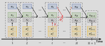
The observable state $\pmb{x}_t$ and latent state $\pmb{z}_t$ are represented by solid and shaded nodes respectively. The directed edges represent causal interactions. At any time period $t+1$, the process state output node $\pmb{s}_{t+1}=(\pmb{x}_{t+1},\pmb{z}_{t+1})$ depends on its parent nodes: $\pmb{s}_{t+1}=\pmb{f}(Pa(\pmb{s}_{t+1});{\pmb\theta}_t)$ with parent nodes $Pa(\pmb{s}_{t+1})=(\pmb{s}_t,\pmb{a}_t,\pmb{e}_{t+1})$ and model parameter $\pmb{\theta}_t=(\pmb{\beta}_t,{V}_{t+1})$.

Complete Hybrid Model Now let’s further incorporate the parametric variations and latent state into hybrid model. Eq.\eqref{eq: 10} becomes

$$ \begin{align} \pmb{x}_{t+1} &=\pmb{g}_x(\pmb{x}_t, \pmb{z}_t, \pmb{a}_t, \pmb{\beta}_t; \pmb{\theta}_t) + \pmb{e}^{x}_{t+1} \\ \pmb{z}_{t+1} &= \pmb{g}_z(\pmb{x}_t, \pmb{z}_t, \pmb{a}_t, \pmb{\beta}_t; \pmb{\theta}_t) + \pmb{e}^{z}_{t+1} ,\end{align} $$ where

• $\pmb{g}_x(\pmb{x}_t, \pmb{z}_t, \pmb{a}_t; \pmb{\beta}_t)\equiv\pmb{x}_t + \Delta t \cdot \pmb{f}_x(\pmb{x}_t,\pmb{z}_t,\pmb{a}_t; \pmb{\beta}_t)$
• $\pmb{g}_z(\pmb{x}_t, \pmb{z}_t, \pmb{a}_t; \pmb{\beta}_t)\equiv\pmb{z}_t + \Delta t \cdot \pmb{f}_z(\pmb{x}_t,\pmb{z}_t,\pmb{a}_t; \pmb{\beta}_t)$,
• $\pmb{e}^{x}_{t+1}\sim \mathcal{N}(0,V^x_{t+1})$, and $\pmb{e}^{z}_{t+1}\sim \mathcal{N}(0,V^z_{t+1})$,
• $\pmb\beta_t\sim \mathcal{N}(\pmb\mu_t^\beta,\Sigma^\beta_t)$.

Inference (A Bayesian Approach)

Observable Process Trajectory

By integrating out latent states $(\pmb{z}_1,\ldots,\pmb{z}_{H+1})$, we have the likelihood of the partially observed trajectory $\pmb\tau_x\equiv (\pmb{x}_1,\pmb{a}_1,\ldots,\pmb{x}_H,\pmb{a}_H,\pmb{x}_{H+1})$, i.e., $$ \begin{equation} p(\pmb{\tau}_x| \pmb\theta)= \int p(\pmb\tau|\pmb\theta) d \pmb{z}_1 \cdots d \pmb{z}_{H+1}\tag{11}\label{eq: 11} \end{equation} $$ Then we can focus on estimating \pmb\theta from the likelihood \eqref{eq: 11} by using approximate Bayesian computation-sequential Monte Carlo (ABC-SMC) method.

ABC-SMC sampling procedure for generating posterior samples from $p(\pmb{\theta}|\mathcal{D})$ (see [7-9]).

Main Idea: Given the observable trajectory $\pmb\tau_x=(\pmb{x}_1,\pmb{a}_1,\ldots,\pmb{x}_H,\pmb{a}_H,\pmb{x}_{H+1})$. $$ \begin{equation} p(\pmb\theta|\pmb\tau_x) \propto p(\pmb\tau_x| \pmb\theta)p(\pmb\theta) \end{equation} $$ The algorithm samples $\pmb\theta$ and $\pmb\tau^\star_x$ from the joint posterior: $$ \begin{equation} p_\delta(\pmb\theta,\pmb\tau_x^\star| \pmb\tau_x)=\frac{p(\pmb\theta)p(\pmb\tau_x^\star|\pmb\theta)\mathbb{1}_\delta[\pmb\tau_x^\star]}{\int\int p(\pmb\theta)p(\pmb\tau^\star_x|\pmb\theta)\mathbb{1}_\delta[\pmb\tau_x^\star]d\pmb\tau_x^\star d\pmb\theta} \end{equation} $$ where $\mathbb{1}_\delta[\pmb\tau_x^\star] = \mathbb{1}_\delta[d(\pmb\tau_x,\pmb\tau_x^\star)\leq \delta]$ is one if $d(\pmb\tau_x,\pmb\tau_x^\star)\leq \delta$ and zero else. When $\delta$ is small, $p_{\delta}(\pmb\theta|\pmb\tau_x)=\int p_\delta(\pmb\theta,\pmb\tau_x^\star| \pmb\tau)d\pmb\tau_x^\star$ is a good approximation to $p(\pmb\theta | \pmb\tau_x)$ because

• When the distance $d(\pmb\tau_x,\pmb\tau_x^\star)\leq \delta$ is small, $\mathbb{1}_\delta[\pmb\tau_x^\star]\rightarrow1$ and Eq.(17) becomes $$ p_\delta(\pmb\theta,\pmb\tau_x^\star| \pmb\tau_x)\rightarrow\frac{p(\pmb\theta)p(\pmb\tau_x^\star|\pmb\theta)}{\int\int p(\pmb\theta)p(\pmb\tau^\star_x|\pmb\theta)d\pmb\tau_x^\star d\pmb\theta}=p(\pmb\theta,\pmb\tau_x^\star|\pmb\tau_x) $$
• Then $p_{\delta}(\pmb\theta|\pmb\tau_x)=\int p_\delta(\pmb\theta,\pmb\tau_x^\star| \pmb\tau)d\pmb\tau^\star_x\rightarrow\int p(\pmb\theta,\pmb\tau_x^\star|\pmb\tau_x)d\pmb\tau^\star_x=p(\pmb\theta|\pmb\tau_x)$

Problem:

1. Low acceptation rate when using the full trajectory $\tau_x$ as summary statistics. It leads to low computational efficiency.
2. Directly compute the distance between simulated and observed trajectories $d(\pmb\tau_x,\pmb\tau_x^\star)$ is computationally expensive and uninformative.Thus instead of directly using trajectory, we can consider sufficient summary statistics of trajectories $\eta(\pmb\tau_x)$ and use the distance measure $d\left(\eta(\tau_x),\eta(\tau^\star_x)\right)$.

New Inference Method: [10] propose a new auxiliary based ABC-SMC method. Check out [10] on arXiv.

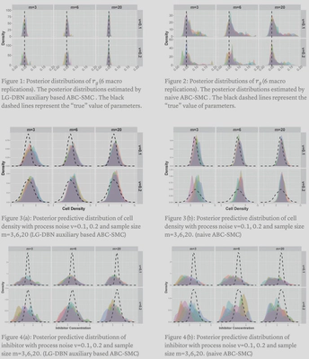
In short, we solved a problem with observable state ($\rho$) and latent variable ($I$) in the following form: $$ \begin{align} \rho_{t+1} &= \rho_t + \Delta t \cdot r_g \rho_t \Bigg (1 - \Big(1+e^{(k_s(k_c-I_t))} \Big) ^{-1} \Bigg ) + e^{\rho}_{t}\\ I_{t+1} &= I_t + \Delta t \cdot \Bigg (\frac{\rho_{t+1}-\rho_t}{\Delta t} - r_d I_t \Bigg) + e^I_t \end{align} $$

We compared two different approximate Bayesian computation method to estimate the posterior distribution $p(\pmb\theta|\mathcal{D})$: LG-DBN auxiliary likelihood-based ABC-SMC approach and naive ABC-SMC.

Conclusion

I briefly reviewed the theoretical basics of dynamic Bayesian network based hybrid model with a short discussion about its inference. I hope this new model class could inspire other researchers to model complex stochastic process in different domain.

Next?

In the next blogs, I will discuss more on (1) the parameter estimation, (2) generalize the model to policy augmented dynamic Bayesian newtork (PADBN) by incoporating reinforcement learning, (3) may provide more interpretability tools such as Shaley value based factor importance (closed form); (4) more about the implementation.

Reference

1. Mockus, L., Peterson, J. J., Lainez, J. M., & Reklaitis, G. V. (2015). Batch-to-batch variation: a key component for modeling chemical manufacturing processes. Organic Process Research & Development, 19(8), 908-914.
2. Vasdekis, A. E., Silverman, A. M., & Stephanopoulos, G. (2015). Origins of cell-to-cell bioprocessing diversity and implications of the extracellular environment revealed at the single-cell level. Scientific Reports, 5(1), 1-7.
3. Dickens, J., Khattak, S., Matthews, T. E., Kolwyck, D., & Wiltberger, K. (2018). Biopharmaceutical raw material variation and control. Current opinion in chemical engineering, 22, 236-243.
4. Zheng, H., Xie, W., Ryzhov, I. O., & Xie, D. (2021). Policy optimization in bayesian network hybrid models of biomanufacturing processes. arXiv preprint arXiv:2105.06543.
5. Murphy, K. P. (2012). Machine learning: a probabilistic perspective. MIT press.
6. Zheng, H., Xie, W., Wang, K., & Li, Z. (2022). Opportunities of Hybrid Model-based Reinforcement Learning for Cell Therapy Manufacturing Process Development and Control. arXiv preprint arXiv:2201.03116.
7. Toni, T., Welch, D., Strelkowa, N., Ipsen, A., & Stumpf, M. P. (2009). Approximate Bayesian computation scheme for parameter inference and model selection in dynamical systems. Journal of the Royal Society Interface, 6(31), 187-202.
8. Lenormand, M., Jabot, F., & Deffuant, G. (2013). Adaptive approximate Bayesian computation for complex models. Computational Statistics, 28(6), 2777-2796.
9. Del Moral, P., Doucet, A., & Jasra, A. (2006). Sequential monte carlo samplers. Journal of the Royal Statistical Society: Series B (Statistical Methodology), 68(3), 411-436.
10. Xie, W., Wang K., Zheng H. & Feng B (2022)Dynamic Bayesian Network Auxiliary ABC-SMC for Hybrid Model Bayesian Inference to Accelerate Biomanufacturing Process Mechanism Learning and Robust Control. arXiv preprint arXiv:2205.02410.